Chaotic Water Wheel
<bgsound src="Midi/mars.mid" loop=infinite>
Objectives
Background
Physical Model
Testing
Exploring the Parameter Space
Deriving equations for our wheel
Second Question
Objectives
· Build a Lorenzian Waterwheel.
· Run tests and confirm the system’s chaotic nature.
· Explore the parameter space of the wheel.
· Derive a system of equations for our specific wheel.
· Using Matlab, solve the system and examine plots.
· Use our experimental data to create the two equations that we were not able to measure experimentally in Matlab.
Top
Background
Chaotic Dynamical Systems
Specifically, chaos is the long term unpredictability of deterministic, nonlinear dynamical systems due to sensitivity to initial conditions. Chaos theory started in 1960 with a professor of meteorology at MIT named Edward Lorenz. Lorenz was running a computer program that modeled weather patterns and created forecasts when he noticed, by chance, that the system he had programmed was severely sensitive to initial conditions. He accidentally changed an initial condition by what could be compared to the effect of the flap of a butterfly’s wings on the global weather pattern. He then saw his system diverge slowly from what it had initially been until it bore no resemblance to the original at all. Lorenz was fascinated with the phenomenon. A while later, while attempting to model the convection patterns of a fluid being heated in a container, Lorenz produced the first ever chaotic dynamical system. He stripped Navier-Stokes equations down to their bones and came up with the following system of first order differential equations:
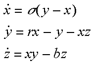
This famous system’s equations represent the rotational speed of the convection, the difference in temperature on either side of the container, and the system’s deviation from a straight line temperature path. The solutions to these equations exhibit very fascinating properties. The thing that makes them "chaotic," however, is their sensitivity to initialconditions. The green graph below is a plot of one of the Lorenz equations with initial conditions [8 1 1]. The blue is the same equation with initial conditions [8 1.000001 1].
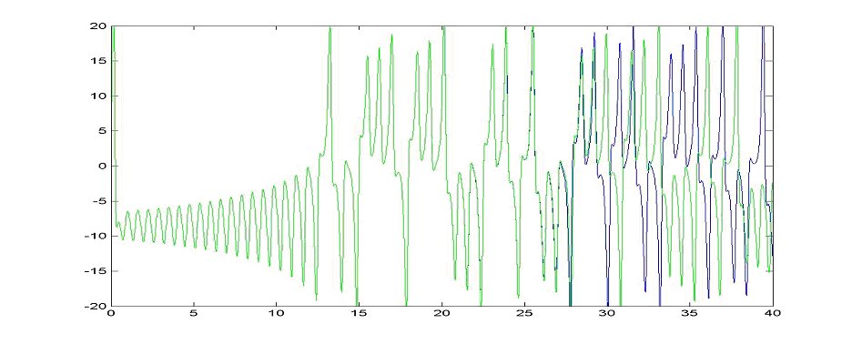
Notice how the two graphs are identical for a while and then eventually bear no similarity at all. This sensitivity is "Chaos." But, the fascinating thing about chaos is that it also exhibits patterns. A phase space plot of the three Lorenz equations produces an image known as a "Strange Attractor." (seen below)
Because the three equations are so codependent, their trajectories orbit back and forth between two centers but never cross. Such properties (combined with the sensitivity to initial conditions) are what makes systems chaotic.
A Lorenzian (or "chaotic") waterwheel is a physical model that perfectly corresponds to the Lorenz equations.A chaotic waterwheel is just like a normal waterwheel except for the facts that he buckets leak. Water pours into the top bucket at a steady rate and gives the system energy while water leaks out of each bucket at a steady rate and removes energy from the system. If the parameters of the wheel are set correctly, the wheel will exhibit chaotic motion: rather than spinning in one direction at a constant speed, the wheel will speed up, slow down, stop, change directions, and oscillate back and forth between combinations of behaviors in an unpredictable manner.

Top
Physical Model
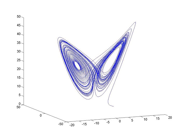
The design for our waterwheel went through many changes. We had access to a rapid-prototyping machine thanks to the college of Mechanical Engineering and we planned to use the machine to manufacture the buckets for our wheel. Unfortunately, the machine was damaged during the semester and was not scheduled for repair until the Spring. Our first few wheel drafts were designed with the rapid-prototyping machine in mind. This first idea had a sort of "ferris wheel" look to it. The design was or a vertical wheel with swiveling buckets like the seats on a ferris wheel. We decided against this design because of our inability to change as many parameters as we thought would be necessary. We needed a way to vary the magnitude of the buckets’ effect on the wheel quickly and easily. With this in mind, our design evolved into a tilted wheel model much like one constructed by Stogatz (seen to the right).
With such a design, we could easily change the tilt of the wheel (thus changing how much the weight in the buckets contributes to the spin of the wheel). We hoped to be able to obtain a turntable for our wheel, but had no luck finding one that fit our specifications. However, we did end up finding two lazy susans of 13 and 18 inch diameters which we decided would fit our purposes. We designed several different buckets to fit the edge of these lazy susans, but with no way to manufacture them, such designs had to also be abandoned. We decided upon using simple plastic cups for buckets.
We built a crude version of our wheel with the smaller of the two lazy susans. We put only 8 cups around the perimeter and ran a few preliminary tests. This first test produced an oscillatory pendulum-type motion. The wheel never turned a complete 360 degrees in either direction, but swung back and forth. After trying several different tilt angles without noticing any different type of behavior, we decided to use the larger wheel and as many cups along the perimeter as possible. We noticed the importance of the system being driven during EVERY second. With cups missing, there were often times when the wheel appeared to almost turn over twice, but then didn’t because a gap in the cups paused under the water flow.
We finally came upon this design: an eighteen inch lazy susan mounted on an adjustable base with 19 cups around the edge.
Unfortunately, the friction in the lazy susan proved to be far too much for the weight of the cups to overcome at ANY tilt angle. When tested, this wheel would spin for a while and would behave as expected as long as its velocity stayed relatively high. But, as soon as the cups on either side started to slow it down, the friction in the lazy susan really kicked in and locked the wheel in place. This, our fourth major design, had to also be trashed.
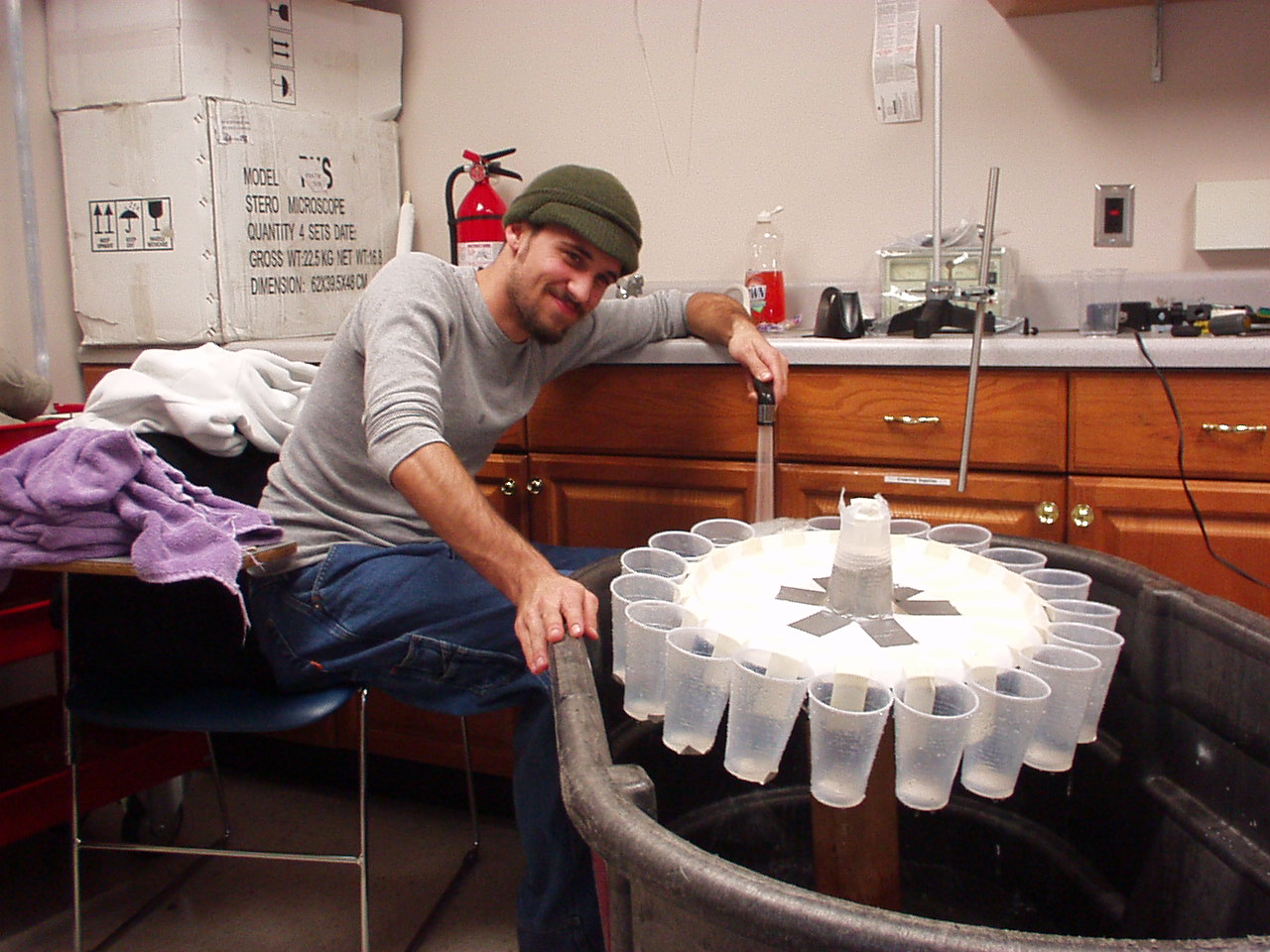
Finally, our design reduced itself to the simplest setup imaginable. A plastic cup’s bottom was cut out and attached to the rotating end of a rotary motion sensor and hung upside down (as though it were pouring water out). Six leaky cups were then attached to the rim of the first cup and the entire apparatus was held up by a ring stand and tilted at the desired angle:
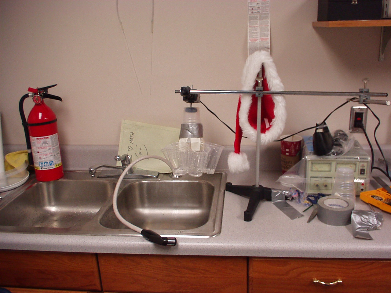
This designed served our purpose quite well and although it was not the precision machine that we had in mind, it displayed all of the properties we desired.
Top
Testing
We ran around twenty tests with varying tilt angles, inflow rates, and leak rates. Ultimately, our wheel achieved three different qualitative behaviors: Rolling Motion, Pendulum Motion, and Chaotic Motion.
Rolling motion can be defined as motion in only one direction. In this type of behavior, the wheel spins in one direction only and never stops or switches direction. We did not keep any data of this type of motion as it is especially uninteresting and is not caused by the parameter range that we are considering.
Quite generally, rolling motion can be achieved by an extremely low or extremely high inflow rate. In the first case, water pours in slowly and the cups leak completely out before reaching the other side of the wheel. In the second case, water pours in so quickly, that the top cup is driven around a full turn and then begins to be filled again.
Pendulum motion is defined as any type of motion that has an obvious periodicity. Our wheel achieved several types of pendulum motion with several different periods. Usually, the wheel would spin less than a full turn in either direction over and over. However, the wheel occasionally settled into a state that repeated itself after oscillating two or three times in either direction.
Examples of both types of pendulum motion are shown below:
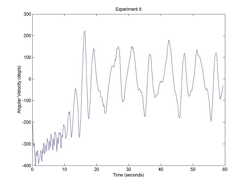
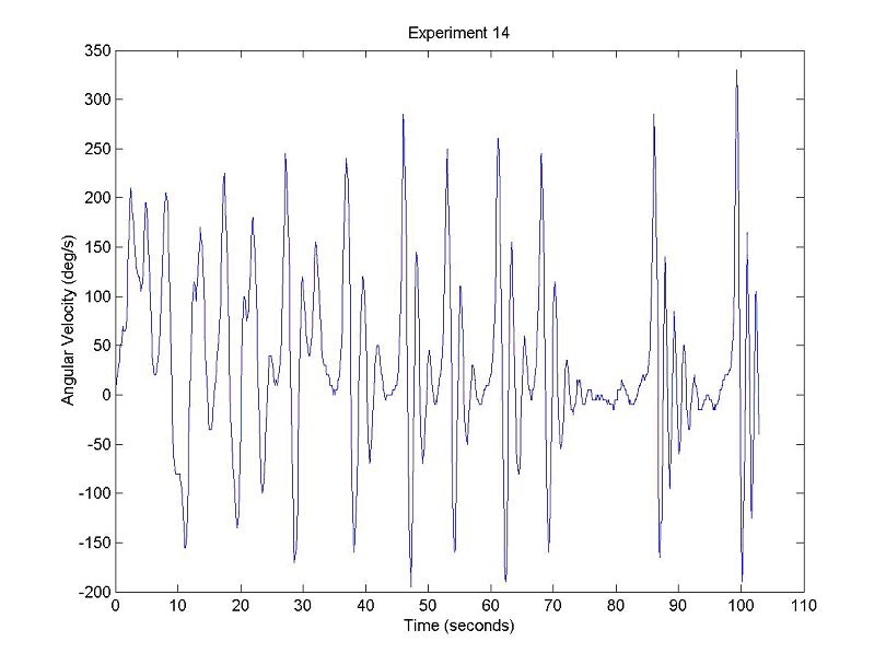
Chaotic motion has no recognizable periodicity or pattern to it. When the wheel is in chaotic spin, it spends no predictable amount of time moving in either direction. Examples are here (view Examples):
Top
Exploring the Parameter Space
The only parameters that we could easily change in our experiments were the inflow rate, and the tilt of the wheel. Changing the leak rate was possible, but tedious, and working with only two parameters at a time simplifies things.
We ran twenty tests and kept all of the data with the exception of the tests that exhibited rolling motion. We rather randomly changed parameters to approximate values (fast water flow, medium fast, medium slow, slow) and recorded the status of the wheel during each run. The following graph explains our results:

The above graph shows the relationship between parameters and wheel behavior. A "C" was placed for chaotic motion, an "R" for rolling motion, and a "P" for periodic motion Please note that the graph is approximate. The states are not placed precisely and the graph is not to scale. However, it does tell us a little bit about our wheel. From our experiment and the rough sketch we have of the parameter space, we can notice that rolling motion is associated with very large water flow rates and very small water flow rates. Periodic behavior is almost completely confined to slower flow rates for all types of tilts, but also pops up at a higher flow rate with a medium tilt. Chaos occurred generally, when the water flow was fast, but not insanely fast. We achieved chaotic motion at every level of tilt. Because we spent so much time trying to put a physical model together, we didn’t have the opportunity to gather as much data in the last few weeks of the semester. Hopefully, we’ll be able to collect more in the spring and perhaps refine this approximation of the parameter space.
Top
Deriving equations for our wheel
The famous Lorenz system of equations is:
This system was intended to model convection in a heated fluid. In this system, x corresponds to the rotational speed of the convection, y corresponds to the difference in temperature on either side of the container, and z corresponds to the system’s deviation from a straight line temperature path. It has been suggested by some that these equations correspond to the rotational velocity of the waterwheel, the difference in the volume of water between the right half and the left half, and the difference in volume between the top half and bottom half. Others say that that the third equation should be the ratio of water volume on the top half of the wheel to that on the bottom half.
Another student’s webpage
(http://kendrick.colgate.edu/mboothe/chaos/) suggests the following system for the behavior of the wheel:
A'=WB-kA
B'= -WB-kW+q
W'=(-vW+pi*g*rad*A)/ u
where
rad= radius of the wheel
k= leakage rate
v= rotational damping rate
u= moment of inertia of the wheel
pi = the value of pie
g= gravitational constant
Our approach was to model only one of the three equations. We decided to attempt to use numerical methods to solve a 2nd order ode that we created for the acceleration of the wheel in terms of position and time. By numerically solving this equation, we would be able to easily prove its chaotic nature.
Sadly, our attempt at numerically solving our 2nd order equation as a system of two first order equations did not work out. We wanted to use the ode45 function in Matlab to solve our equation, but we ran into a serious problem. We had to meet such conditions as water leaking from buckets only when the buckets have water in them. Simulating such circumstances required us to use many types of vector operations in Matlab along with a few for loops. However, the ode45 function is not vector valued. It takes in a function, a time interval, and initial conditions, picks its own step size, and then returns a solution in vector form. This means that any of our vector operations would not go through the ode45 function. This meant we had to express all of our strange periodic piecewise functions explicitly...with no ifs, ands, or buts as they say (more on how we did this in the description of our equation derivation). We ended up having to make quite a few simplifying assumptions that changed our system too drastically for the result to be accurate. Matlab solved our simplified version of the acceleration equation and returned sinusoidal functions. Any attempts to change the qualitative nature of the numerical solutions by altering parameters failed. We concluded that the simplified model was just too far from the correct model for this approach to be successful. The simplified version of our m file along with some of Matlab’s solutions to it is included at the end of this report.
Top
Second Question
Obtain Missing Equations From Experimental Data
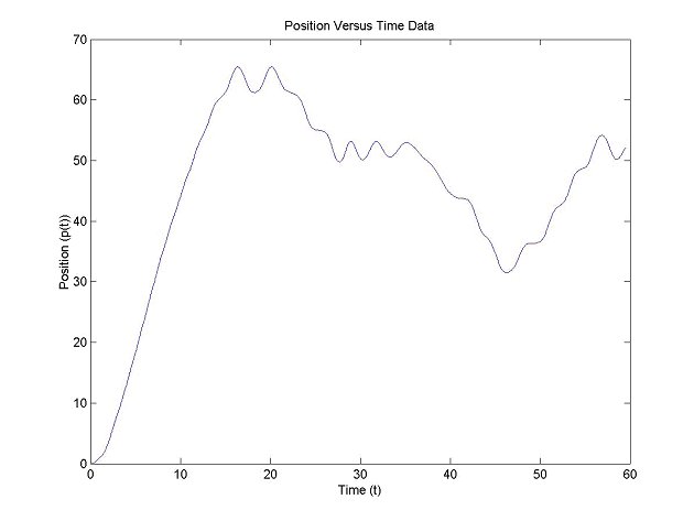
Because we obtained experimental data of velocity versus time graphs, we essentially have sample solutions to one of the three equations that describe our wheel. Our second question involves attempting to use this data to create the missing two equations. The logic behind it is this: If we have data for velocity versus time, we can obtain position versus time by integrating. If we have position versus time, that means that we can calculate the exact position of each bucket at any instant. If we know the position of each bucket at each instant, we know whether or not water is flowing into it. If we know whether or not water is flowing into each bucket at every time step, we know the total volume of each bucket at each time step. The remaining two equations are (according to some) functions only of how much water is on either side of the wheel.
However, we would be required to know the exact relationship between inflow and leakage. Because we have data from a specific system, our initial conditions and parameters must match that system exactly in order for us to be able to find the correct corresponding equations.
The two parameters that must be perfect are inflow rate and leak rate. If we screw one of these up, our new equations will make no sense. If our inflow is too large and our leak too small, we will create an equation that indicates more water on the wrong side of the wheel at some time. Because the three equations are all codependent, our equation for velocity and our equation for the difference in water volume on either side must match up. There must be more water on one side of the wheel when the velocity is increasing, and more water on the other when velocity is increasing. (This type of relationship led us to some interesting conclusions which will be discussed later).
There is hope. We already have the capability to know exactly how much water flowsinto each bucket and when. Because we created functions like this:
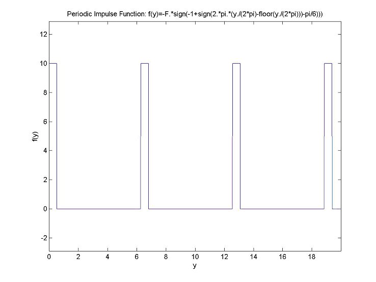
that express inflow in terms of position, and because we have specific data for position in terms of time:
We can create inflow versus time in the following manner:
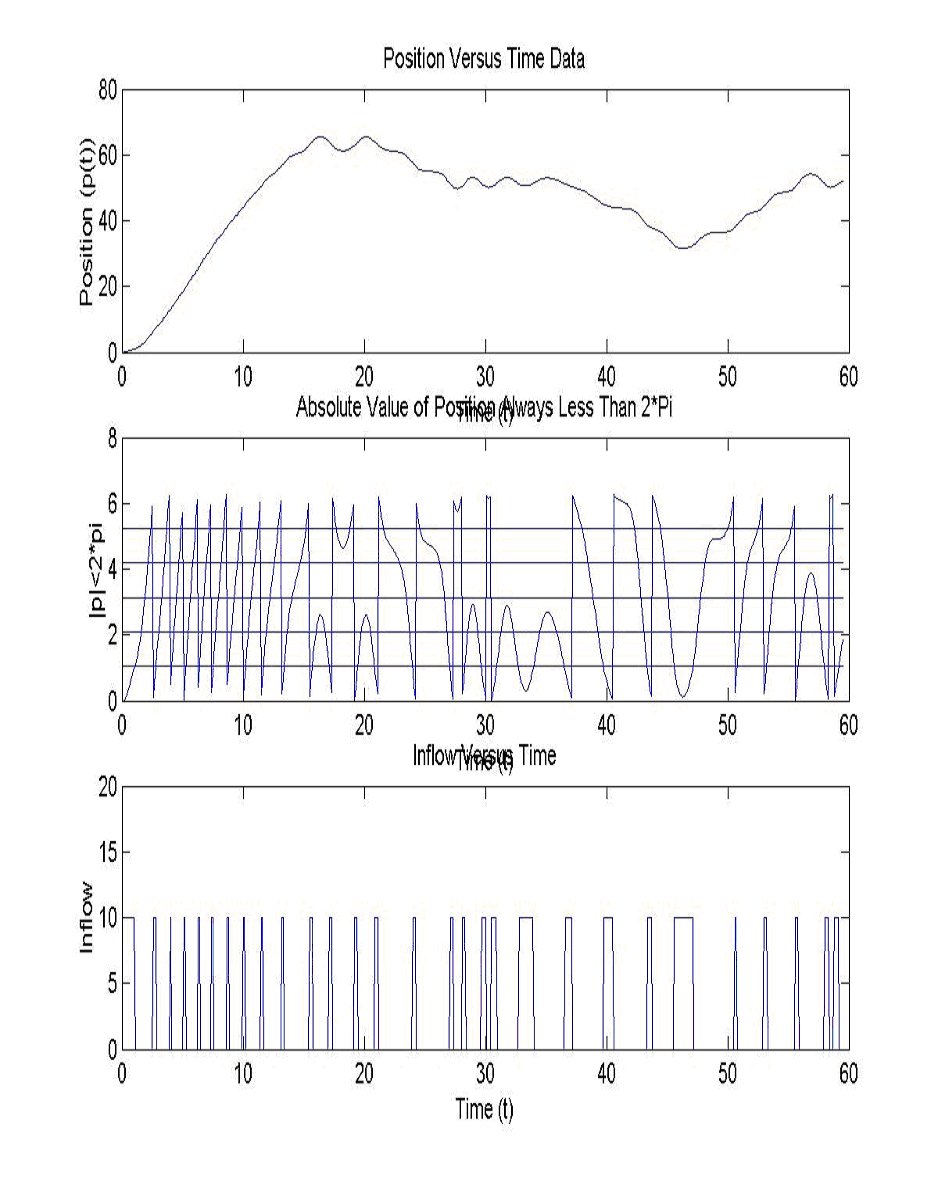
This means we have a specific inflow versus time function for each position versus time function. We know exactly when water is flowing into what bucket. The only thing we don’t know for certain is how fast it leaks out. We can make the inflow rate whatever we want as long as our leakage rate is correctly scaled to match.
Using this knowledge, we can create "inflow rate into the right half" and "inflow rate into the left half" functions of time. We must now consider what conditions have to be met in order for the functions for "total water in the right half" and "total water in the left half" to be correct. The conditions are as follows. Neglecting damping, the weight of the water is the only thing accelerating the wheel. Therefore, when the wheel’s acceleration is zero, the affects of the water must be zero. This means that for our correct inflow and leakage rates, the maxima and minima of the acceleration function must match up with the zeros of the right-left function. (This is quite interesting because it follows that the right-left function serves exactly as a scaled derivative of the acceleration function if the system has no damping.)
Meeting these criteria has proved to be most challenging and we are still attempting to find an efficient way to find correct inflow and leakage rates. Nevertheless, the process we created even without the correct initial conditions has produced some pretty interesting results. The process is exactly as described above:
· Use velocity versus time to create position versus time.
· Use position versus time to create inflow versus time.
· Use inflow versus time along with some leakage rate to create left, right, top and bottom functions.
· Combine left, right, top, and bottom functions as necessary.
Considering that our initial conditions were off, the results were quite good. There is an obvious relationship between the frequency of the oscillations in the functions we created and those of the acceleration function. Plotting all three equations against one another did not create a pretty butterfly attractor, but did manage to show us something with noticeable centers of symmetry. You can see the trajectory being pulled toward a center even if the center isn’t very clear. The following is a sample of what our process created:
Top